
tala
Technical Analysis Library for Assets
tala is a TypeScript technical analysis library for
OHLC price history. You build a chain of indicators with
tala(), call .run(history) once, and get
back a cloned array enriched with calculated fields. No mutation,
no globals, zero runtime dependencies, and full CJS + ESM output.
What this library covers
| Category | Indicators |
|---|---|
| Moving averages | SMA, EMA, WEMA, ALMA, TRIX |
| Momentum | MACD, RSI, CCI, ADX, Fisher Transform, Stochastic, Williams %R, Stochastic RSI |
| Volatility | Bollinger Bands, ATR |
| Volume | OBV, VWAP |
| Price levels | Pivot Points, Fibonacci Retracement Levels |
| Signals | MACD Cross, RSI Cross, CCI Cross, ALMA Cross, Fisher Cross |
How to read these docs
If this is your first time, read in order: Install → Quick Start → How It Works. Each indicator section that follows is self-contained and includes the formula, a worked numeric example where helpful, and an interpretation guide.
history[0] is the most recent
bar. 2) When a bar does not have enough lookback history, the
indicator field is set to 0 (or omitted for keyed
outputs) instead of throwing.
Install
npm install @jimzandueta/talaQuick Start
This example starts with a small OHLC price history array, runs a
few indicators, and shows the resulting enriched values returned by
.run().
1. Create a sample price history
The newest bar is at index 0 (see Overview for the
convention).
import { tala } from '@jimzandueta/tala'

const priceHistory = [
  { date: '2026-01-05', open: 104, high: 110, low: 100, close: 105 },
  { date: '2026-01-04', open: 99,  high: 108, low: 98,  close: 102 },
  { date: '2026-01-03', open: 96,  high: 105, low: 95,  close: 98 },
  { date: '2026-01-02', open: 92,  high: 98,  low: 91,  close: 95 },
  { date: '2026-01-01', open: 88,  high: 94,  low: 87,  close: 90 }
]
2. Run indicators
The chain below calculates sma3, ema3, and
rsi3 for each bar where enough lookback data exists.
const result = tala()
  .sma(3)
  .ema(3)
  .rsi(3)
  .run(priceHistory)
3. Read the enriched result
.run() returns a new enriched array. The original
priceHistory array is not mutated.
result[0]
// {
 //   date: '2026-01-05',
 //   open: 104,
 //   high: 110,
 //   low: 100,
 //   close: 105,
 //   sma3: 101.66666666666667,
 //   ema3: 101.58333333333334,
 //   changeVal: 3,
 //   rsi3: 100
// }(105 + 102 + 98) / 3 = 101.67
(98 + 95 + 90) / 3 = 94.33; then
bar 1 = 98.17; then bar 0 = 101.58
0 and RSI resolves
to 100
4. Full output shape
The resulting array keeps the same order as the input and appends calculated fields to each entry.
[
  {
    date: '2026-01-05',
    close: 105,
    sma3: 101.66666666666667,
    ema3: 101.58333333333334,
    changeVal: 3,
    rsi3: 100
  },
  {
    date: '2026-01-04',
    close: 102,
    sma3: 98.33333333333333,
    ema3: 98.16666666666667,
    changeVal: 4,
    rsi3: 100
  },
  {
    date: '2026-01-03',
    close: 98,
    sma3: 94.33333333333333,
    ema3: 94.33333333333333,
    changeVal: 3,
    rsi3: 0
  },
  {
    date: '2026-01-02',
    close: 95,
    sma3: 0,
    ema3: 0,
    changeVal: 5,
    rsi3: 0
  },
  {
    date: '2026-01-01',
    close: 90,
    sma3: 0,
    ema3: 0,
    changeVal: 0,
    rsi3: 0
  }
]
Structured output with signals
Use { structured: true } when you want the enriched
history and grouped signal events returned separately.
const { history, signals } = tala()
  .sma(3)
  .rsi(3)
  .rsiCross()
  .run(priceHistory, { structured: true })

history[0].sma3
// 101.66666666666667

signals.rsiCross
// [
 //   {
 //     date: '2026-01-05',
 //     open: 104,
 //     high: 110,
 //     low: 100,
 //     close: 105,
 //     sma3: 101.66666666666667,
 //     changeVal: 3,
 //     rsi3: 100
 //   }
 // ]
How It Works
tala() returns a TalaChain. Each method
(.sma(), .ema(), .macd(),
...) appends one operation to a queue and returns the chain so calls
can be chained. Nothing is computed until
.run(history) is called.
At .run() time, tala deep-clones the history, executes
each queued operation in order, and writes its outputs onto every
bar where enough lookback exists. Indicators that depend on others
(for example, MACD reads two EMAs internally; ADX reads TR and DM
through a WEMA) handle their own dependencies — you only chain what
you actually want surfaced on the result.
.run() on any number of datasets.
changeVal.
.rsi() computes the close-to-close diff internally; you
do not need to pre-process it.
{ structured: true } to
.run() to also receive grouped cross-signal events
under signals.
Charting
chart() is a terminal chain method that renders your computed indicators
with TradingView Lightweight Charts.
HTML mode
Writes a self-contained HTML file to disk. Open it directly in any browser (no local server required).
await tala()
  .sma(14)
  .ema(26)
  .bb(20, 2)
  .macd()
  .rsi(14)
  .chart(history, { format: 'html' })
The generated page includes:
- Candlestick chart with overlay indicators (SMA, EMA, Bollinger Bands, etc.)
- Oscillator panes grouped by scale: 0–100 (RSI, ADX, Stoch), around 0 (MACD, Williams %R, Fisher), and CCI
- Per-pane hover tooltips with OHLC and indicator values
- Sidebar legend with per-indicator visibility toggles
- Optional time-scale sync across panes
- Editable OHLCV table (candles update immediately as you edit)
- PNG export for the full chart layout (via html2canvas)
Server mode
Starts a local HTTP server and opens your browser automatically. In this mode, Recalculate is enabled: edit OHLCV values in the data table, click the button, and tala re-runs the chain on the server with the updated data. If the requested port is busy, tala tries the next available port.
await tala()
  .sma(14)
  .rsi(14)
  .chart(history, { format: 'server', port: 7890 })
Chart rendering requires this peer dependency:
npm install lightweight-charts
# Generate a demo chart
npx tsx demo/test-viz.ts

# Or start the live server
npx tsx demo/test-server.ts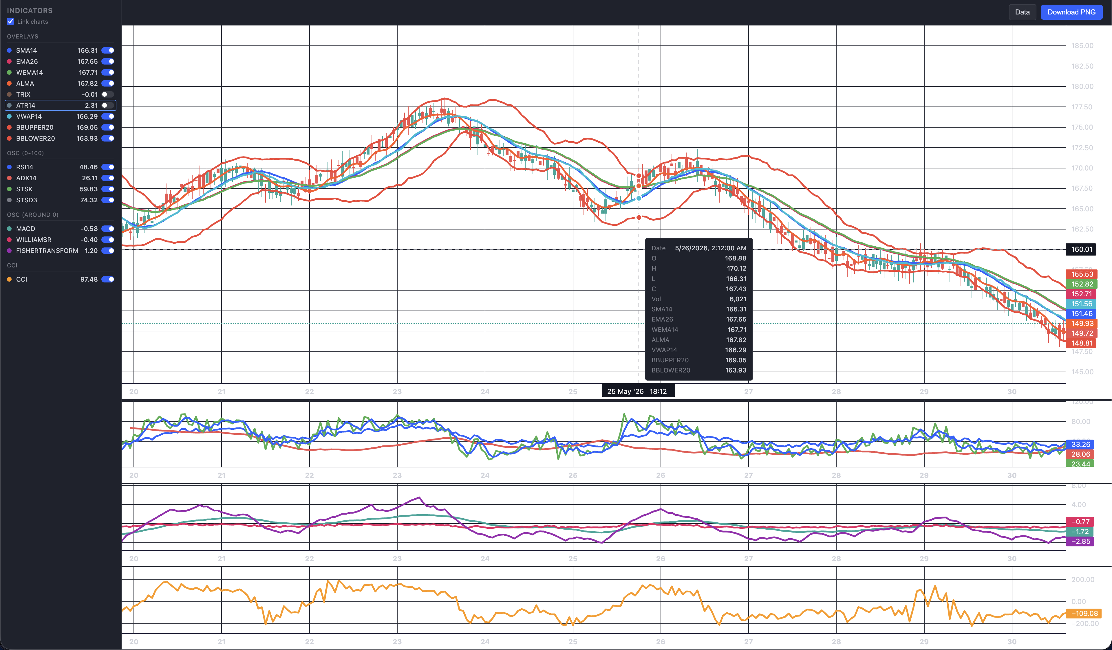
| Option | Type | Default | Description |
|---|---|---|---|
format | 'html' | 'server' | 'server' | Output mode |
filePath | string | './demo/tala-chart.html' | Output path for HTML mode |
port | number | 7890 | Port for server mode |
title | string | 'tala chart' | Chart title |
Simple Moving Average -
.sma(period, priceKey?, setKey?)
Arithmetic mean of the last n closing prices. Writes
sma{period} (e.g. sma14). Entries without
enough history are set to 0.
| Index | Close | sma3 |
|---|---|---|
| 0 (newest) | 105 | (105 + 102 + 98) / 3 = 101.67 |
| 1 | 102 | (102 + 98 + 95) / 3 = 98.33 |
| 2 | 98 | (98 + 95 + 90) / 3 = 94.33 |
| 3 | 95 | 0 (not enough history) |
| 4 (oldest) | 90 | 0 |
tala().sma(14).run(history)
// result[0].sma14 → number
Exponential Moving Average -
.ema(period, offset?, priceKey?, setKey?)
Weighted average giving more importance to recent prices. Seeded
from the SMA at the oldest valid bar, then propagated forward.
Writes ema{period}.
tala().ema(12).run(history)
// result[0].ema12 → number
Wilder's EMA -
.wema(period, offset, priceKey?, setKey?)
Same recursive structure as EMA but uses a smoothing factor of $1/n$
(half the speed of a standard EMA). Also called RMA or Wilder's
Smoothing. Used internally by ADX. Writes wema{period}.
tala().wema(14, 0).run(history)
// result[0].wema14 → number
ALMA - .alma(period?, sigma?, offset?, priceKey?)
Arnaud Legoux Moving Average. Uses a Gaussian (bell-curve) weight
distribution so the smoothing peak can be positioned closer to
recent bars, reducing lag without adding noise. Writes
alma. Defaults: period=9, sigma=6, offset=0.85.
tala().alma().run(history)           // period=9, sigma=6, offset=0.85
tala().alma(20, 6, 0.9).run(history)  // custom: period=20, less lag
// result[0].alma → number
TRIX - .trix(period?, priceKey?, setKey?)
Triple-smoothed EMA rate of change. Applies EMA
three times to filter short-term noise, then outputs the 1-bar
percentage change. Values oscillate around zero — positive = upward
momentum. Writes trix. Default period=18.
tala().trix(18).run(history)
// result[0].trix → number (% rate-of-change of EMA3, oscillates ≈ 0)
MACD - .macd(periods?, options?, priceKey?, setKey?)
Moving Average Convergence Divergence. Measures momentum as the
difference between a fast and slow EMA. Positive
= fast EMA above slow EMA (bullish). Optionally writes
signal (EMA of MACD) and histogram.
Defaults: fast=12, slow=26, signalLength=9.
tala()
  .macd(
    { fastPeriod: 12, slowPeriod: 26, signalLength: 9 },
    { includeSignal: true, includeHistogram: true }
  )
  .run(history)
// result[0].macd      → EMA12 − EMA26
// result[0].signal    → 9-period EMA of MACD
// result[0].histogram → MACD − Signal
RSI - .rsi(period?, changeKey?, setKey?)
Relative Strength Index. Measures speed and magnitude of price
changes. Values 0-100; above 70 = overbought, below 30 = oversold.
changeVal is computed automatically. Writes
rsi{period}. Default period=14.
tala().rsi(14).run(history)
// result[0].rsi14 → 0-100
CCI - .cci(period?, constant?, priceKeys?, setKey?)
Commodity Channel Index. Measures how far the typical price deviates
from its rolling mean, scaled by mean absolute deviation. Above +100
= overbought; below −100 = oversold. Writes cci.
Defaults: period=20, constant=0.015.
tala().cci(20).run(history)
// result[0].cci → number (typically −200 to +200)
ADX - .adx(period?, priceKeys?, setKey?)
Average Directional Index. Measures trend strength (not
direction) on a 0-100 scale. Below 20 = ranging; above 25 = strong
trend. Pair with di+ / di- for direction.
Internally uses WEMA smoothing of
TR (true range) and +DM/-DM
(directional movement). Default period=14.
tala().adx(14).run(history)
// result[0].adx14  → 0-100 (trend strength)
// result[0]['di+'] → +DI (bullish directional pressure)
// result[0]['di-'] → -DI (bearish directional pressure)
// result[0].atr14  → Average True Range
Fisher Transform -
.fisher(period?, priceKeys?, setKeys?)
Converts price into a Gaussian normal distribution using a Fisher
transformation, making turning points sharper and easier to spot.
Writes fisherTransform and
fisherSignal (previous bar's transform). Default
period=9.
tala().fisher().run(history)
// result[0].fisherTransform → number (sharp turning-point indicator)
// result[0].fisherSignal    → previous bar's fisherTransform
Stochastic Oscillator -
.sts(period?, priceKeys?, setKey?)
Compares the current close to the high-low range over the lookback
period. Values 0-100; above 80 = overbought, below 20 = oversold.
Writes stsK (%K line) and stsD3 (3-period
SMA of %K = %D line). Default period=14.
tala().sts().run(history)
// result[0].stsK  → %K (0-100)
// result[0].stsD3 → %D - 3-period SMA of %K
Williams %R - .williamsR(period?, priceKeys?, setKey?)
Inverse of the Stochastic %K — measures where the current close sits within the recent high-low range, negated. Range 0 to −1 (this library scales the standard −100 to 0 range by dividing by 100). Near 0 = overbought; near −1 = oversold. Default period=14.
tala().williamsR().run(history)
// result[0].williamsR → 0 to −1  (0 = overbought, −1 = oversold)
Pivot Points - .pivotT(period?, priceKeys?)
Traditional pivot points computed from the previous
period-bar chunk, then written onto the current chunk.
This matches the standard pivot convention of using prior-period
high, low, and close. Writes pp{period},
r1{period}, s1{period},
r2{period}, s2{period}. Default period=20.
tala().pivotT(20).run(history)
// result[0].pp20  → Pivot Point
// result[0].r120  → Resistance 1   result[0].s120  → Support 1
// result[0].r220  → Resistance 2   result[0].s220  → Support 2
Fibonacci Retracements - .fibRL(period?, priceKeys?)
Fibonacci-style levels derived from the
pivot band. In this library they are computed
by interpolating between s2{period} and
r2{period} after pivot points are generated internally.
This is a library-specific level construction, not the more common
PP ± r × range notation. Default period=20.
s2 to r2, descending from
r2 as r increases.
tala().fibRL(20).run(history)
// result[0]['fib0.236'] → number
// result[0]['fib0.382'] → number
// result[0]['fib0.5']   → midpoint
// result[0]['fib0.618'] → golden ratio level
// result[0]['fib0.786'] → number
Stochastic RSI - .stochRSI(period?, changeKey?, kSetKey?, dSetKey?)
Applies the Stochastic formula to the RSI series rather than to raw price.
The K line measures where the current RSI sits within the RSI high/low range over
the lookback window. Default period=14. changeVal is computed automatically
if not already present.
tala().stochRSI(14).run(history)
// result[0].stochRSIK → K line (0–100)
// result[0].stochRSID3 → D line (3-bar SMA of K)
Bollinger Bands - .bb(period?, k?, priceKey?)
A volatility envelope centered on a simple moving average. The upper and lower bands are placed k population standard deviations above and below the mean. Default period=20, k=2, priceKey='close'.
tala().bb(20).run(history)
// result[0].bbUpper20 → upper band
// result[0].bbMid20   → middle band (SMA)
// result[0].bbLower20 → lower band
ATR (Average True Range) - .atr(period?, priceKeys?, setKey?)
Measures market volatility as the Wilder-smoothed average of the True Range. True Range is the greatest of: current high minus low, absolute distance from previous close to current high, and absolute distance from previous close to current low. Default period=14.
tala().atr(14).run(history)
// result[0].atr14 → ATR value
// result[0].tr    → True Range of each bar
OBV (On-Balance Volume) - .obv(priceKey?, volumeKey?, setKey?)
Cumulative running total of volume, signed by the direction of the price move.
When price is up, volume is added; when down, volume is subtracted; when unchanged,
OBV is carried forward. Missing volume is treated as 0.
tala().obv().run(history)
// result[0].obv → cumulative OBV value
VWAP (Volume-Weighted Average Price) - .vwap(period?, priceKeys?, volumeKey?, setKey?)
Rolling volume-weighted average price computed over a sliding window.
Each bar's weight is its volume; the price used is the Typical Price (H+L+C)/3.
Missing volume is treated as 0, and the fallback is the plain TP of the
anchor bar. Default period=14.
tala().vwap(14).run(history)
// result[0].vwap14 → VWAP value for the 14-bar window
Cross Signals
Cross signals identify the exact bars where one value crosses
another value or threshold. They are useful for converting indicator
output into discrete events such as bullish,
bearish, overbought, or
oversold signals.
What counts as a cross?
A cross happens when the relationship between two values changes from the previous bar to the current bar.
Supported cross helpers
| Method | Purpose | Typical signal |
|---|---|---|
.macdCross() |
Detects when the MACD line crosses the MACD signal line. | Momentum shift |
.rsiCross() |
Detects RSI threshold crossings, commonly around 70 and 30. | Overbought or oversold transition |
.cciCross() |
Detects CCI crosses through a configurable level, commonly
around 100 or -100.
|
Momentum threshold break |
.almaCross() |
Detects when price crosses the ALMA line. | Price versus trend-line shift |
.fisherCross() |
Detects when Fisher Transform crosses its signal line. | Short-term reversal timing cue |
Signal output shape
Signal arrays return the matching enriched price-history entries. That means each signal item keeps the original OHLC fields and includes whichever indicator fields were calculated before the signal helper ran.
type PriceHistoryEntry = {
  date?: string
  open: number
  high: number
  low: number
  close: number

  // Added by indicators depending on the chain
  sma20?: number
  sma50?: number
  ema12?: number
  ema26?: number
  macd?: number
  signal?: number
  histogram?: number
  rsi14?: number
  changeVal?: number

  // The object may include additional calculated fields
  // based on the indicators used in your chain.
}signals
contains enriched bars, not separate tiny event objects.
MACD cross — .macdCross()
.macdCross() is used after calculating MACD with a
signal line. It checks when macd crosses above or below
signal.
macd crosses
above signal. This usually means upside momentum is
increasing.
macd crosses
below signal. This usually means upside momentum is
weakening or downside momentum is increasing.
histogram = macd - signal.
const { history, signals } = tala()
  .macd(
    { fastPeriod: 12, slowPeriod: 26, signalLength: 9 },
    { includeSignal: true, includeHistogram: true }
  )
  .macdCross()
  .run(priceHistory, { structured: true })

signals.macdCross
// [
 //   {
 //     date: '2026-01-18',
 //     open: 118,
 //     high: 124,
 //     low: 116,
 //     close: 123,
 //     ema12: 116.42,
 //     ema26: 113.08,
 //     macd: 3.34,
 //     signal: 2.91,
 //     histogram: 0.43
 //   }
 // ]
RSI cross — .rsiCross()
.rsiCross() is used after calculating RSI. It is
commonly used to detect crosses around overbought and oversold
thresholds.
| Threshold | Meaning | Common interpretation |
|---|---|---|
70 |
Overbought zone | RSI crossing down from above 70 may suggest momentum cooling. |
30 |
Oversold zone | RSI crossing up from below 30 may suggest downside pressure is easing. |
50 |
Midline | RSI crossing above 50 can indicate bullish momentum bias; crossing below 50 can indicate bearish bias. |
const { history, signals } = tala()
  .rsi(14)
  .rsiCross()
  .run(priceHistory, { structured: true })

signals.rsiCross
// [
 //   {
 //     date: '2026-01-12',
 //     open: 104,
 //     high: 108,
 //     low: 99,
 //     close: 101,
 //     changeVal: -5,
 //     rsi14: 68.42
 //   }
 // ]
Additional supported helpers
tala also includes cross helpers for CCI, ALMA, and Fisher Transform. These follow the same structured-output pattern as MACD and RSI crosses: calculate the indicator first, then add the cross helper at the end of the chain.
| Method | Prerequisite indicator | Event logic |
|---|---|---|
.cciCross() |
.cci() |
CCI crossing a level such as 100. |
.almaCross() |
.alma() |
Close price crossing the ALMA line. |
.fisherCross() |
.fisher() |
Fisher Transform crossing its signal line. |
const { history, signals } = tala()
  .cci(20)
  .alma(20, 6, 0.9)
  .fisher()
  .cciCross()
  .almaCross(20, 6, 0.9)
  .fisherCross()
  .run(priceHistory, { structured: true })

signals.cciCross
// [
 //   {
 //     date: '2026-01-20',
 //     open: 126,
 //     high: 131,
 //     low: 124,
 //     close: 130,
 //     cci: 114.28
 //   }
 // ]

signals.almaCross
signals.fisherCross
Structured output
When .run() is called with
{ structured: true }, tala returns both the enriched
price history and a grouped signals object.
const output = tala()
  .sma(14)
  .rsi(14)
  .macd({ fastPeriod: 12, slowPeriod: 26, signalLength: 9 }, { includeSignal: true })
  .macdCross()
  .rsiCross()
  .run(priceHistory, { structured: true })

output.history
// Enriched PriceHistoryEntry[] with calculated indicator fields

output.signals
// {
 //   macdCross: [
 //     {
 //       date: '2026-01-18',
 //       open: 118,
 //       high: 124,
 //       low: 116,
 //       close: 123,
 //       sma14: 116.86,
 //       rsi14: 61.74,
 //       macd: 3.34,
 //       signal: 2.91
 //     }
 //   ],
 //   rsiCross: [
 //     {
 //       date: '2026-01-12',
 //       open: 104,
 //       high: 108,
 //       low: 99,
 //       close: 101,
 //       sma14: 109.42,
 //       rsi14: 68.42,
 //       macd: 1.88,
 //       signal: 2.04
 //     }
 //   ]
 // }
Unstructured output
When structured is omitted or set to
false, .run() returns the enriched history
array directly.
const enriched = tala()
  .rsi(14)
  .rsiCross()
  .run(priceHistory)

enriched[0]
// Most recent enriched bar
Example signal workflow
A practical workflow is to calculate indicators first, then add cross signals at the end of the chain.
const chain = tala()
  .sma(20)
  .sma(50)
  .rsi(14)
  .macd(
    { fastPeriod: 12, slowPeriod: 26, signalLength: 9 },
    { includeSignal: true, includeHistogram: true }
  )
  .rsiCross()
  .macdCross()

const { history, signals } = chain.run(priceHistory, { structured: true })
Best practices
.macd(...) before .macdCross().
Common Parameters
Most indicators accept the same set of optional parameters for
customising input fields and output keys. They make tala work with
arbitrary candle shapes (e.g. c/h/l
instead of close/high/low)
and let you write multiple instances of the same indicator into
different keys.
| Parameter | Type | Default | Purpose |
|---|---|---|---|
priceKey |
string |
'close' |
Single input field. Used by indicators that read one price per bar (SMA, EMA, WEMA, ALMA, TRIX, MACD, histogram). |
priceKeys |
PriceKeys |
{ c: 'close', h: 'high', l: 'low' } |
OHLC field-name mapping. Used by indicators that need high/low/close (CCI, ADX, Fisher, Stochastic, Williams %R, pivotT, fibRL, TR, DM, TP). |
setKey |
string |
indicator-specific (e.g. 'sma',
'rsi', 'cci')
|
Base name of the output field written onto each entry. For
period-aware indicators the period is appended (e.g.
sma14, rsi14, wema14).
For period-less indicators the base name is written as-is.
|
setKey (Stochastic) |
STSSetKey |
{ k: 'stsK', d: 'stsD' } |
Output keys for %K and %D lines. |
setKeys (Fisher) |
FisherSetKeys |
{ t: 'fisherTransform', s: 'fisherSignal' }
|
Output keys for the transform and the signal (previous bar's transform). |
changeKey |
string |
'changeVal' |
Field that holds the close-to-close change. Used by RSI; auto-computed when missing. |
Renaming the output — setKey
Use setKey to compute the same indicator twice with
different parameters and keep both results.
const result = tala()
  .sma(14)
  .sma(14, 'volume', 'volSma')   // SMA(14) of volume → volSma14
  .ema(12, 0, 'close', 'fastEma') // EMA(12) of close → fastEma12
  .run(history)

result[0].sma14      // default close-SMA(14)
result[0].volSma14   // volume-SMA(14)
result[0].fastEma12 // renamed EMA(12)setKey (so
setKey: 'fastEma' with period=12 writes
fastEma12). Indicators without a period (CCI, ADX base
output, Williams %R, ALMA, TRIX, Fisher) write the base name as-is.
Custom OHLC field names — priceKey /
priceKeys
If your data uses short names like
c/h/l or domain-specific
names, override the defaults instead of remapping your data.
// Candles with short field names
const history = [
  { o: 104, h: 110, l: 100, c: 105 },
  { o: 100, h: 108, l: 98,  c: 102 },
  // ...
]

tala()
  .sma(14, 'c')                                  // priceKey = 'c'
  .cci(20, 0.015, { c: 'c', h: 'h', l: 'l' })  // priceKeys
  .adx(14, { c: 'c', h: 'h', l: 'l' })
  .run(history)
Stochastic and Fisher — multi-output keys
Stochastic writes two keys (%K, %D) and Fisher writes two keys (transform, signal). Pass an object to override the defaults.
tala()
  .sts(14, { c: 'close', h: 'high', l: 'low' }, { k: 'stochK', d: 'stochD' })
  .fisher(9, { c: 'close', h: 'high', l: 'low' }, { t: 'fisher', s: 'fisherPrev' })
  .run(history)

result[0].stochK       // renamed %K
result[0].stochD3      // renamed %D (period appended)
result[0].fisher       // renamed transform
result[0].fisherPrev   // renamed signal
RSI — changeKey
RSI consumes changeVal (close-to-close difference). It
is auto-computed if missing, so you only need
changeKey if you have a pre-computed change field under
a different name.
tala()
  .rsi(14)                          // reads/writes default 'changeVal'
  .rsi(14, 'myDelta', 'rsiCustom') // reads 'myDelta', writes rsiCustom14
  .run(history)
Quick reference — defaults per indicator
| Indicator | Reads | Writes (default) |
|---|---|---|
.sma(period, priceKey?, setKey?) |
close |
sma{period} |
.ema(period, offset?, priceKey?, setKey?) |
close |
ema{period} |
.wema(period, offset, priceKey?, setKey?) |
close |
wema{period} |
.alma(period?, sigma?, offset?, priceKey?) |
close |
alma |
.trix(period?, priceKey?, setKey?) |
close |
trix |
.macd(periods?, options?, priceKey?, setKey?)
|
close |
macd (+ signal,
histogram)
|
.rsi(period?, changeKey?, setKey?) |
changeVal |
rsi{period} |
.cci(period?, constant?, priceKeys?, setKey?)
|
high, low, close |
cci |
.adx(period?, priceKeys?, setKey?) |
high, low, close |
adx{period}, di+, di-,
atr{period}
|
.fisher(period?, priceKeys?, setKeys?) |
high, low |
fisherTransform, fisherSignal |
.sts(period?, priceKeys?, setKey?) |
high, low, close |
stsK, stsD{period} |
.williamsR(period?, priceKeys?, setKey?) |
high, low, close |
williamsR |
.pivotT(period?, priceKeys?) |
high, low, close |
pp{p}, r1{p}, s1{p}, r2{p}, s2{p} |
.fibRL(period?, priceKeys?) |
high, low, close |
fib0.236 … fib0.786 |
Types
import type {
  PriceHistoryEntry,   // candle shape (open, high, low, close, ...)
  PriceKeys,           // { c, h, l } - field name mapping
  MACDPeriods,         // { fastPeriod, slowPeriod, signalLength }
  MACDOptions,         // { includeSignal?, includeHistogram? }
  STSSetKey,           // { k, d } - output key names for Stochastic
  FisherSetKeys,       // { t, s } - output key names for Fisher
  TalaResult,          // { history, signals } - structured run() output
  RunOptions,          // { structured?: boolean }
} from '@jimzandueta/tala'
Utilities
getTrend(priceHist, key, start?, end?, isVector?)
Returns 1 (uptrend), -1 (downtrend), or
0 (sideways) by computing the linear regression slope
over the selected window. Does not mutate the array. Imported
directly - not on the chain.
import { getTrend } from '@jimzandueta/tala'

const dir = getTrend(history, 'close')           // 1 | -1 | 0
const dir = getTrend(history, 'sma14', 0, 20)    // over the first 20 bars
Input Format
All indicators expect PriceHistoryEntry[] where
index 0 is the most recent candle (reverse
chronological order).
interface PriceHistoryEntry {
  open:       number
  high:       number
  low:        number
  close:      number
  volume?:    number
  changeVal?: number   // close[i] − close[i+1]; auto-computed by .rsi()
  [key: string]: number | undefined
}